21. Statistical Divergence Measures#

21.1. Overview#

A statistical divergence quantifies discrepancies between two distinct probability distributions that can be challenging to distinguish for the following reason:

• every event that has positive probability under one of the distributions also has positive probability under the other distribution

• this means that there is no “smoking gun” event whose occurrence tells a statistician that one of the probability distributions surely governs the data

A statistical divergence is a function that maps two probability distributions into a nonnegative real number.

Statistical divergence functions play important roles in statistics, information theory, and what many people now call “machine learning”.

This lecture describes three divergence measures:

• Kullback–Leibler (KL) divergence

• Jensen–Shannon (JS) divergence

• Chernoff entropy

These will appear in several quantecon lectures.

Let’s start by importing the necessary Python tools.

import matplotlib.pyplot as plt
import numpy as np
from numba import vectorize, jit
from math import gamma
from scipy.integrate import quad
from scipy.optimize import minimize_scalar
import pandas as pd
from IPython.display import display, Math

21.2. Primer on entropy, cross-entropy, KL divergence#

Before diving in, we’ll introduce some useful concepts in a simple setting.

We’ll temporarily assume that $f$ and $g$ are two probability mass functions for discrete random variables on state space $I=\{1,2,\dots ,n\}$ that satisfy $f_i\ge 0,\sum _i{f}_i=1,g_i\ge 0,\sum _i{g}_i=1$.

We follow some statisticians and information theorists who define the surprise or surprisal associated with having observed a single draw $x=i$ from distribution $f$ as

They then define the information that you can anticipate to gather from observing a single realization as the expected surprisal

Claude Shannon [Shannon, 1948] called $H(f)$ the entropy of distribution $f$.

Kullback and Leibler [Kullback and Leibler, 1951] define the amount of information that a single draw of $x$ provides for distinguishing $f$ from $g$ as the log likelihood ratio

The following two concepts are widely used to compare two distributions $f$ and $g$.

Cross-Entropy:

Kullback-Leibler (KL) Divergence:

These concepts are related by the following equality.

To prove (21.3), note that

Remember that $H(f)$ is the anticipated surprisal from drawing $x$ from $f$.

Then the above equation tells us that the KL divergence is an anticipated “excess surprise” that comes from anticipating that $x$ is drawn from $f$ when it is actually drawn from $g$.

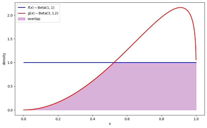
21.3. Two Beta distributions: running example#

We’ll use Beta distributions extensively to illustrate concepts.

The Beta distribution is particularly convenient as it’s defined on $[0,1]$ and exhibits diverse shapes by appropriately choosing its two parameters.

The density of a Beta distribution with parameters $a$ and $b$ is given by

Let’s define parameters and density functions in Python

# Parameters in the two Beta distributions
F_a, F_b = 1, 1
G_a, G_b = 3, 1.2

@vectorize
def p(x, a, b):
    r = gamma(a + b) / (gamma(a) * gamma(b))
    return r * x** (a-1) * (1 - x) ** (b-1)

# The two density functions
f = jit(lambda x: p(x, F_a, F_b))
g = jit(lambda x: p(x, G_a, G_b))

# Plot the distributions
x_range = np.linspace(0.001, 0.999, 1000)
f_vals = [f(x) for x in x_range]
g_vals = [g(x) for x in x_range]

plt.figure(figsize=(10, 6))
plt.plot(x_range, f_vals, 'b-', linewidth=2, label=r'$f(x) \sim \text{Beta}(1,1)$')
plt.plot(x_range, g_vals, 'r-', linewidth=2, label=r'$g(x) \sim \text{Beta}(3,1.2)$')

# Fill overlap region
overlap = np.minimum(f_vals, g_vals)
plt.fill_between(x_range, 0, overlap, alpha=0.3, color='purple', label='overlap')

plt.xlabel('x')
plt.ylabel('density')
plt.legend()
plt.show()

21.4. Kullback–Leibler divergence#

Our first divergence function is the Kullback–Leibler (KL) divergence.

For probability densities (or pmfs) $f$ and $g$ it is defined by

We can interpret $D_{KL}(f\Vert g)$ as the expected excess log loss (expected excess surprisal) incurred when we use $g$ while the data are generated by $f$.

It has several important properties:

• Non-negativity (Gibbs’ inequality): $D_{KL}(f\Vert g)\ge 0$ with equality if and only if $f=g$ almost everywhere.

• Asymmetry: $D_{KL}(f\Vert g)\ne D_{KL}(g\Vert f)$ in general (hence it is not a metric)

• Information decomposition: $D_{KL}(f\Vert g)=H(f,g)-H(f)$, where $H(f,g)$ is the cross entropy and $H(f)$ is the Shannon entropy of $f$.

• Chain rule: For joint distributions $f(x,y)$ and $g(x,y)$, $D_{KL}(f(x,y)\Vert g(x,y))=D_{KL}(f(x)\Vert g(x))+E_f[D_{KL}(f(y|x)\Vert g(y|x))]$

KL divergence plays a central role in statistical inference, including model selection and hypothesis testing.

Likelihood Ratio Processes describes a link between KL divergence and the expected log likelihood ratio, and the lecture A Problem that Stumped Milton Friedman connects it to the test performance of the sequential probability ratio test.

Let’s compute the KL divergence between our example distributions $f$ and $g$.

def compute_KL(f, g):
    """
    Compute KL divergence KL(f, g) via numerical integration
    """
    def integrand(w):
        fw = f(w)
        gw = g(w)
        return fw * np.log(fw / gw)
    val, _ = quad(integrand, 1e-5, 1-1e-5)
    return val

# Compute KL divergences between our example distributions
kl_fg = compute_KL(f, g)
kl_gf = compute_KL(g, f)

print(f"KL(f, g) = {kl_fg:.4f}")
print(f"KL(g, f) = {kl_gf:.4f}")

KL(f, g) = 0.7590
KL(g, f) = 0.3436

The asymmetry of KL divergence has important practical implications.

$D_{KL}(f\Vert g)$ penalizes regions where $f>0$ but $g$ is close to zero, reflecting the cost of using $g$ to model $f$ and vice versa.

21.5. Jensen-Shannon divergence#

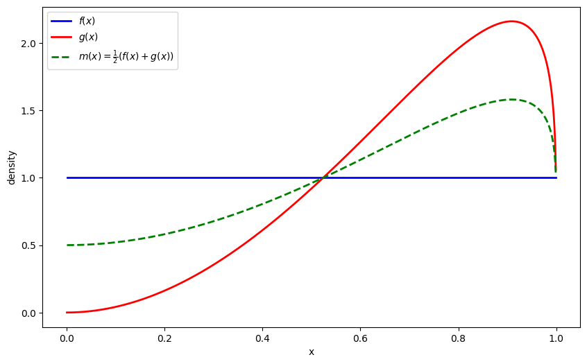
Sometimes we want a symmetric measure of divergence that captures the difference between two distributions without favoring one over the other.

This often arises in applications like clustering, where we want to compare distributions without assuming one is the true model.

The Jensen-Shannon (JS) divergence symmetrizes KL divergence by comparing both distributions to their mixture:

where $m$ is a mixture distribution that averages $f$ and $g$

Let’s also visualize the mixture distribution $m$:

def m(x):
    return 0.5 * (f(x) + g(x))

m_vals = [m(x) for x in x_range]

plt.figure(figsize=(10, 6))
plt.plot(x_range, f_vals, 'b-', linewidth=2, label=r'$f(x)$')
plt.plot(x_range, g_vals, 'r-', linewidth=2, label=r'$g(x)$')
plt.plot(x_range, m_vals, 'g--', linewidth=2, label=r'$m(x) = \frac{1}{2}(f(x) + g(x))$')

plt.xlabel('x')
plt.ylabel('density')
plt.legend()
plt.show()

The JS divergence has several useful properties:

• Symmetry: $JS(f,g)=JS(g,f)$.

• Boundedness: $0\le JS(f,g)\le \log 2$.

• Its square root $\sqrt{JS}$ is a metric (Jensen–Shannon distance) on the space of probability distributions.

• JS divergence equals the mutual information between a binary random variable $Z\sim \text{Bernoulli}(1/2)$ indicating the source and a sample $X$ drawn from $f$ if $Z=0$ or from $g$ if $Z=1$.

The Jensen–Shannon divergence plays a key role in the optimization of certain generative models, as it is bounded, symmetric, and smoother than KL divergence, often providing more stable gradients for training.

Let’s compute the JS divergence between our example distributions $f$ and $g$

def compute_JS(f, g):
    """Compute Jensen-Shannon divergence."""
    def m(w):
        return 0.5 * (f(w) + g(w))
    js_div = 0.5 * compute_KL(f, m) + 0.5 * compute_KL(g, m)
    return js_div

js_div = compute_JS(f, g)
print(f"Jensen-Shannon divergence JS(f,g) = {js_div:.4f}")

Jensen-Shannon divergence JS(f,g) = 0.0984

We can easily generalize to more than two distributions using the generalized Jensen-Shannon divergence with weights $\alpha =({\alpha }_i{)}_{i=1}^n$:

where:

• ${\alpha }_i\ge 0$ and $\sum _{i=1}^n{\alpha }_i=1$, and

• $H(f)=-\int f(x)\log f(x)dx$ is the Shannon entropy of distribution $f$

21.6. Chernoff entropy#

Chernoff entropy originates from early applications of the theory of large deviations, which refines central limit approximations by providing exponential decay rates for rare events.

For densities $f$ and $g$ the Chernoff entropy is

Remarks:

• The inner integral is the Chernoff coefficient.

• At $\varphi =1/2$ it becomes the Bhattacharyya coefficient $\int \sqrt{fg}$.

• In binary hypothesis testing with $T$ iid observations, the optimal error probability decays as $e^{-C(f,g)T}$.

We will see an example of the third point in the lecture Likelihood Ratio Processes, where we study the Chernoff entropy in the context of model selection.

Let’s compute the Chernoff entropy between our example distributions $f$ and $g$.

def chernoff_integrand(ϕ, f, g):
    """Integral entering Chernoff entropy for a given ϕ."""
    def integrand(w):
        return f(w)**ϕ * g(w)**(1-ϕ)
    result, _ = quad(integrand, 1e-5, 1-1e-5)
    return result

def compute_chernoff_entropy(f, g):
    """Compute Chernoff entropy C(f,g)."""
    def objective(ϕ):
        return chernoff_integrand(ϕ, f, g)
    result = minimize_scalar(objective, bounds=(1e-5, 1-1e-5), method='bounded')
    min_value = result.fun
    ϕ_optimal = result.x
    chernoff_entropy = -np.log(min_value)
    return chernoff_entropy, ϕ_optimal

C_fg, ϕ_optimal = compute_chernoff_entropy(f, g)
print(f"Chernoff entropy C(f,g) = {C_fg:.4f}")
print(f"Optimal ϕ = {ϕ_optimal:.4f}")

Chernoff entropy C(f,g) = 0.1212
Optimal ϕ = 0.5969

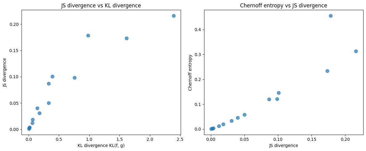
21.7. Comparing divergence measures#

We now compare these measures across several pairs of Beta distributions

distribution_pairs = [
    # (f_params, g_params)
    ((1, 1), (0.1, 0.2)),
    ((1, 1), (0.3, 0.3)),
    ((1, 1), (0.3, 0.4)),
    ((1, 1), (0.5, 0.5)),
    ((1, 1), (0.7, 0.6)),
    ((1, 1), (0.9, 0.8)),
    ((1, 1), (1.1, 1.05)),
    ((1, 1), (1.2, 1.1)),
    ((1, 1), (1.5, 1.2)),
    ((1, 1), (2, 1.5)),
    ((1, 1), (2.5, 1.8)),
    ((1, 1), (3, 1.2)),
    ((1, 1), (4, 1)),
    ((1, 1), (5, 1))
]

# Create comparison table
results = []
for i, ((f_a, f_b), (g_a, g_b)) in enumerate(distribution_pairs):
    f = jit(lambda x, a=f_a, b=f_b: p(x, a, b))
    g = jit(lambda x, a=g_a, b=g_b: p(x, a, b))
    kl_fg = compute_KL(f, g)
    kl_gf = compute_KL(g, f)
    js_div = compute_JS(f, g)
    chernoff_ent, _ = compute_chernoff_entropy(f, g)
    results.append({
        'Pair (f, g)': f"\\text{{Beta}}({f_a},{f_b}), \\text{{Beta}}({g_a},{g_b})",
        'KL(f, g)': f"{kl_fg:.4f}",
        'KL(g, f)': f"{kl_gf:.4f}",
        'JS': f"{js_div:.4f}",
        'C': f"{chernoff_ent:.4f}"
    })

df = pd.DataFrame(results)
# Sort by JS divergence
df['JS_numeric'] = df['JS'].astype(float)
df = df.sort_values('JS_numeric').drop('JS_numeric', axis=1)

columns = ' & '.join([f'\\text{{{col}}}' for col in df.columns])
rows = ' \\\\\n'.join(
    [' & '.join([f'{val}' for val in row]) 
     for row in df.values])

latex_code = rf"""
\begin{{array}}{{lcccc}}
{columns} \\
\hline
{rows}
\end{{array}}
"""

display(Math(latex_code))

We can clearly see co-movement across the divergence measures as we vary the parameters of the Beta distributions.

Next we visualize relationships among KL, JS, and Chernoff entropy.

kl_fg_values = [float(result['KL(f, g)']) for result in results]
js_values = [float(result['JS']) for result in results]
chernoff_values = [float(result['C']) for result in results]

fig, axes = plt.subplots(1, 2, figsize=(12, 5))

axes[0].scatter(kl_fg_values, js_values, alpha=0.7, s=60)
axes[0].set_xlabel('KL divergence KL(f, g)')
axes[0].set_ylabel('JS divergence')
axes[0].set_title('JS divergence vs KL divergence')

axes[1].scatter(js_values, chernoff_values, alpha=0.7, s=60)
axes[1].set_xlabel('JS divergence')
axes[1].set_ylabel('Chernoff entropy')
axes[1].set_title('Chernoff entropy vs JS divergence')

plt.tight_layout()
plt.show()

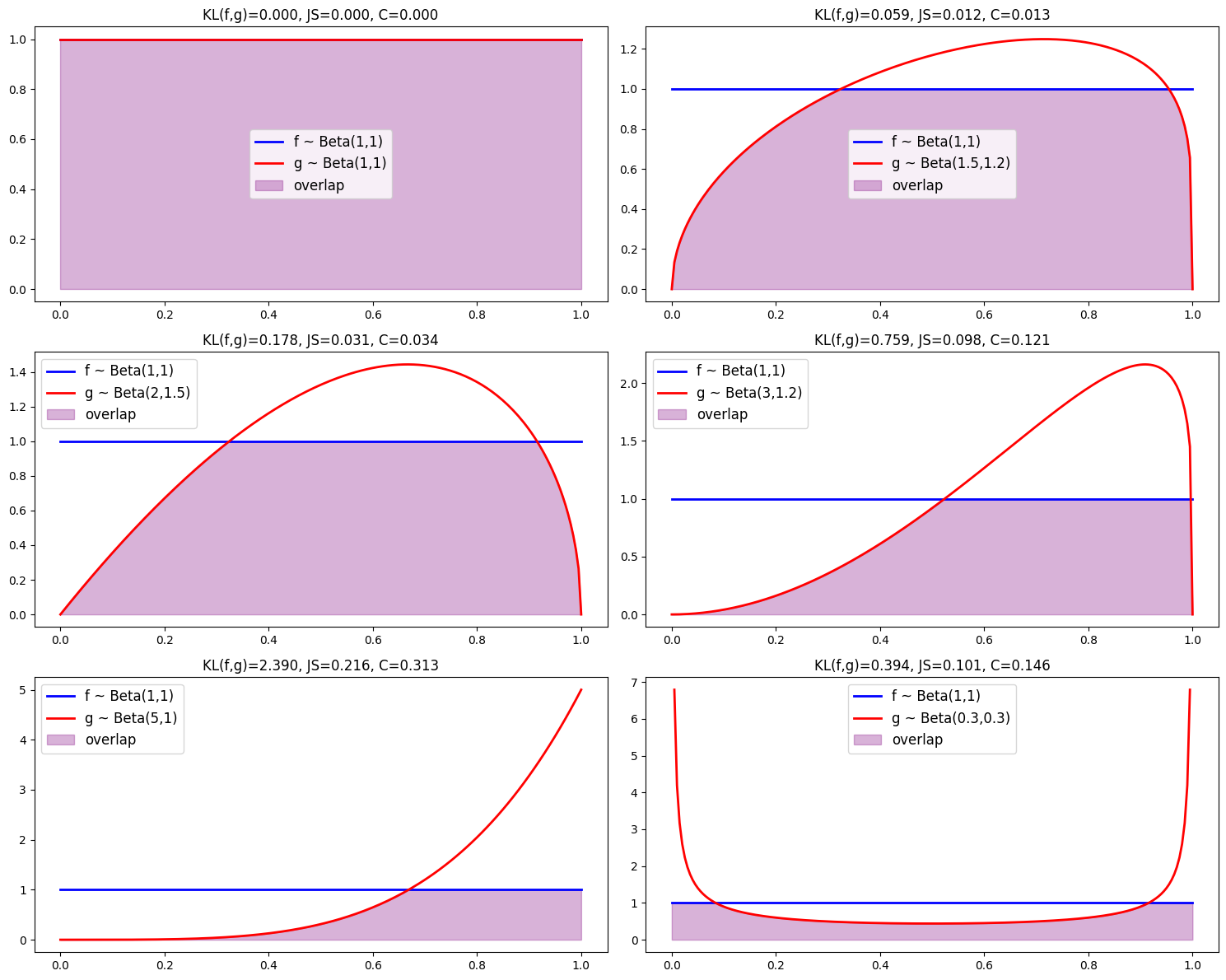
We now generate plots illustrating how overlap visually diminishes as divergence measures increase.

param_grid = [
    ((1, 1), (1, 1)),   
    ((1, 1), (1.5, 1.2)),
    ((1, 1), (2, 1.5)),  
    ((1, 1), (3, 1.2)),  
    ((1, 1), (5, 1)),
    ((1, 1), (0.3, 0.3))
]

Show code cell source

Hide code cell source

def plot_dist_diff(para_grid):
    """Plot overlap of selected Beta distribution pairs."""

    fig, axes = plt.subplots(3, 2, figsize=(15, 12))
    divergence_data = []
    for i, ((f_a, f_b), (g_a, g_b)) in enumerate(param_grid):
        row, col = divmod(i, 2)
        f = jit(lambda x, a=f_a, b=f_b: p(x, a, b))
        g = jit(lambda x, a=g_a, b=g_b: p(x, a, b))
        kl_fg = compute_KL(f, g)
        js_div = compute_JS(f, g)
        chernoff_ent, _ = compute_chernoff_entropy(f, g)
        divergence_data.append({
            'f_params': (f_a, f_b),
            'g_params': (g_a, g_b),
            'kl_fg': kl_fg,
            'js_div': js_div,
            'chernoff': chernoff_ent
        })
        x_range = np.linspace(0, 1, 200)
        f_vals = [f(x) for x in x_range]
        g_vals = [g(x) for x in x_range]
        axes[row, col].plot(x_range, f_vals, 'b-', 
                        linewidth=2, label=f'f ~ Beta({f_a},{f_b})')
        axes[row, col].plot(x_range, g_vals, 'r-', 
                        linewidth=2, label=f'g ~ Beta({g_a},{g_b})')
        overlap = np.minimum(f_vals, g_vals)
        axes[row, col].fill_between(x_range, 0, 
                        overlap, alpha=0.3, color='purple', label='overlap')
        axes[row, col].set_title(
            f'KL(f,g)={kl_fg:.3f}, JS={js_div:.3f}, C={chernoff_ent:.3f}', 
            fontsize=12)
        axes[row, col].legend(fontsize=12)
    plt.tight_layout()
    plt.show()
    return divergence_data

divergence_data = plot_dist_diff(param_grid)

21.8. KL divergence and maximum-likelihood estimation#

Given a sample of $n$ observations $X=\{x_1,x_2,\dots ,x_n\}$, the empirical distribution is

where $\delta (x-x_i)$ is the Dirac delta function centered at $x_i$:

• Discrete probability measure: Assigns probability $\frac{1}{n}$ to each observed data point

• Empirical expectation: $⟨X{⟩}_{p_e}=\frac{1}{n}\sum _{i=1}^n{x}_i=\overline{\mu }$

• Support: Only on the observed data points $\{x_1,x_2,\dots ,x_n\}$

The KL divergence from the empirical distribution $p_e$ to a parametric model $p_{\theta }(x)$ is:

Using the mathematics of the Dirac delta function, it follows that

Since the log-likelihood function for parameter $\theta$ is:

it follows that maximum likelihood chooses parameters to minimize

Thus, MLE is equivalent to minimizing the KL divergence from the empirical distribution to the statistical model $p_{\theta }$.

21.9. Related lectures#

This lecture has introduced tools that we’ll encounter elsewhere.

• Other quantecon lectures that apply connections between divergence measures and statistical inference include Likelihood Ratio Processes, A Problem that Stumped Milton Friedman, and Incorrect Models.

• Statistical divergence functions also take center stage in Heterogeneous Beliefs and Financial Markets that studies Lawrence Blume and David Easley’s model of heterogeneous beliefs and financial markets.