7. Using Newton’s Method to Solve Economic Models #

Contents

Using Newton’s Method to Solve Economic Models

7.1. Overview #

Many economic problems involve finding fixed points or zeros (also called “roots”) of functions.

For example, in a simple supply and demand model, an equilibrium price is one that makes excess demand zero.

In other words, an equilibrium is a zero of the excess demand function.

There are various computational techniques for solving for fixed points and zeros.

In this lecture we study an important gradient-based technique called Newton’s method.

Newton’s method does not always work but, in situations where it does, convergence is often fast when compared to other methods.

The lecture will apply Newton’s method in one-dimensional and multidimensional settings to solve fixed-point and zero-finding problems.

When finding the fixed point of a function $f$ , Newton’s method updates an existing guess of the fixed point by solving for the fixed point of a linear approximation to the function $f$ .
When finding the zero of a function $f$ , Newton’s method updates an existing guess by solving for the zero of a linear approximation to the function $f$ .

To build intuition, we first consider an easy, one-dimensional fixed point problem where we know the solution and solve it using both successive approximation and Newton’s method.

Then we apply Newton’s method to multidimensional settings to solve market for equilibria with multiple goods.

At the end of the lecture, we leverage the power of automatic differentiation in jax to solve a very high-dimensional equilibrium problem

We use the following imports in this lecture

import matplotlib.pyplot as plt
from typing import NamedTuple
from scipy.optimize import root
import jax.numpy as jnp
import jax

# Enable 64-bit precision
jax.config.update("jax_enable_x64", True)

7.2. Fixed point computation using Newton’s method #

In this section we solve the fixed point of the law of motion for capital in the setting of the Solow growth model.

We will inspect the fixed point visually, solve it by successive approximation, and then apply Newton’s method to achieve faster convergence.

7.2.1. The Solow model#

In the Solow growth model, assuming Cobb-Douglas production technology and zero population growth, the law of motion for capital is

(7.1)#

k_{t + 1} = g (k_{t}) where g (k) := s A k^{α} + (1 - δ) k

Here

$k_{t}$ is capital stock per worker,
$A, α > 0$ are production parameters, $α < 1$
$s > 0$ is a savings rate, and
$δ \in (0, 1)$ is a rate of depreciation

In this example, we wish to calculate the unique strictly positive fixed point of $g$ , the law of motion for capital.

In other words, we seek a $k^{*} > 0$ such that $g (k^{*}) = k^{*}$ .

such a $k^{*}$ is called a steady state, since $k_{t} = k^{*}$ implies $k_{t + 1} = k^{*}$ .

Using pencil and paper to solve $g (k) = k$ , you will be able to confirm that

k^{*} = {(\frac{s A}{δ})}^{1 / (1 - α)}

7.2.2. Implementation#

Let’s store our parameters in NamedTuple to help us keep our code clean and concise.

class SolowParameters(NamedTuple):
    A: float
    s: float
    α: float
    δ: float

This function creates a suitable SolowParameters with default parameter values.

def create_solow_params(A=2.0, s=0.3, α=0.3, δ=0.4):
    """Creates a Solow model parameterization with default values."""
    return SolowParameters(A=A, s=s, α=α, δ=δ)

The next two functions implement the law of motion (7.1) and store the true fixed point $k^{*}$ .

def g(k, params):
    A, s, α, δ = params
    return A * s * k**α + (1 - δ) * k


def exact_fixed_point(params):
    A, s, α, δ = params
    return ((s * A) / δ) ** (1 / (1 - α))

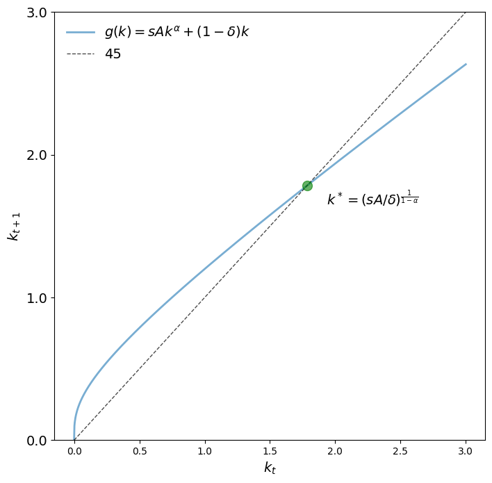
Here is a function to provide a 45 degree plot of the dynamics.

def plot_45(params, ax, fontsize=14):

    k_min, k_max = 0.0, 3.0
    k_grid = jnp.linspace(k_min, k_max, 1200)

    # Plot the functions
    lb = r"$g(k) = sAk^{\alpha} + (1 - \delta)k$"
    ax.plot(k_grid, g(k_grid, params), lw=2, alpha=0.6, label=lb)
    ax.plot(k_grid, k_grid, "k--", lw=1, alpha=0.7, label="45")

    # Show and annotate the fixed point
    kstar = exact_fixed_point(params)
    fps = (kstar,)
    ax.plot(fps, fps, "go", ms=10, alpha=0.6)
    ax.annotate(
        r"$k^* = (sA / \delta)^{\frac{1}{1-\alpha}}$",
        xy=(kstar, kstar),
        xycoords="data",
        xytext=(20, -20),
        textcoords="offset points",
        fontsize=fontsize,
    )

    ax.legend(loc="upper left", frameon=False, fontsize=fontsize)

    ax.set_yticks((0, 1, 2, 3))
    ax.set_yticklabels((0.0, 1.0, 2.0, 3.0), fontsize=fontsize)
    ax.set_ylim(0, 3)
    ax.set_xlabel("$k_t$", fontsize=fontsize)
    ax.set_ylabel("$k_{t+1}$", fontsize=fontsize)

Let’s look at the 45 degree diagram for two parameterizations.

params = create_solow_params()
fig, ax = plt.subplots(figsize=(8, 8))
plot_45(params, ax)
plt.show()

_images/85d461cc659ae25494a959f41aa822d0588b3451b21eb158a7a1d5a425ec4a31.png

params = create_solow_params(α=0.05, δ=0.5)
fig, ax = plt.subplots(figsize=(8, 8))
plot_45(params, ax)
plt.show()

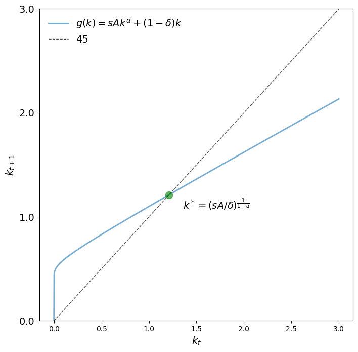
_images/2ef2ce14b6af582e0aba79580381f84da4eba1bacc58a9542a96b41c0520ab4b.png

We see that $k^{*}$ is indeed the unique positive fixed point.

7.2.2.1. Successive approximation#

First let’s compute the fixed point using successive approximation.

In this case, successive approximation means repeatedly updating capital from some initial state $k_{0}$ using the law of motion.

Here’s a time series from a particular choice of $k_{0}$ .

def compute_iterates(k_0, f, params, n=25):
    """Compute time series of length n generated by arbitrary function f."""
    k = k_0
    k_iterates = []
    for t in range(n):
        k_iterates.append(k)
        k = f(k, params)
    return k_iterates

params = create_solow_params()
k_0 = 0.25
k_series = compute_iterates(k_0, g, params)
k_star = exact_fixed_point(params)

fig, ax = plt.subplots()
ax.plot(k_series, "o")
ax.plot([k_star] * len(k_series), "k--")
ax.set_ylim(0, 3)
plt.show()

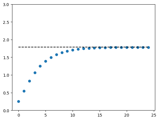
_images/4fb251cfa0b503c9b3a0f1f4ddfd29297d79ec248385e5f9998ab321bdbaff91.png

Let’s see the output for a long time series.

k_series = compute_iterates(k_0, g, params, n=10_000)
k_star_approx = k_series[-1]
k_star_approx

1.7846741842265788

This is close to the true value.

k_star

1.7846741842265788

7.2.2.2. Newton’s method#

In general, when applying Newton’s fixed point method to some function $g$ , we start with a guess $x_{0}$ of the fixed point and then update by solving for the fixed point of a tangent line at $x_{0}$ .

To begin with, we recall that the first-order approximation of $g$ at $x_{0}$ (i.e., the first order Taylor approximation of $g$ at $x_{0}$ ) is the function

(7.2)#

\hat{g} (x) \approx g (x_{0}) + g^{'} (x_{0}) (x - x_{0})

We solve for the fixed point of $\hat{g}$ by calculating the $x_{1}$ that solves

x_{1} = \frac{g (x_{0}) - g^{'} (x_{0}) x_{0}}{1 - g^{'} (x_{0})}

Generalising the process above, Newton’s fixed point method iterates on

(7.3)#

x_{t + 1} = \frac{g (x_{t}) - g^{'} (x_{t}) x_{t}}{1 - g^{'} (x_{t})}, x_{0} given

To implement Newton’s method we observe that the derivative of the law of motion for capital (7.1) is

(7.4)#

g^{'} (k) = α s A k^{α - 1} + (1 - δ)

Let’s define this:

def Dg(k, params):
    A, s, α, δ = params
    return α * A * s * k ** (α - 1) + (1 - δ)

Here’s a function $q$ representing (7.3).

def q(k, params):
    return (g(k, params) - Dg(k, params) * k) / (1 - Dg(k, params))

Now let’s plot some trajectories.

def plot_trajectories(
    params,
    k0_a=0.8,  # first initial condition
    k0_b=3.1,  # second initial condition
    n=20,      # length of time series
    fs=14,     # fontsize
):

    fig, axes = plt.subplots(2, 1, figsize=(10, 6))
    ax1, ax2 = axes

    ks1 = compute_iterates(k0_a, g, params, n)
    ax1.plot(ks1, "-o", label="successive approximation")

    ks2 = compute_iterates(k0_b, g, params, n)
    ax2.plot(ks2, "-o", label="successive approximation")

    ks3 = compute_iterates(k0_a, q, params, n)
    ax1.plot(ks3, "-o", label="newton steps")

    ks4 = compute_iterates(k0_b, q, params, n)
    ax2.plot(ks4, "-o", label="newton steps")

    for ax in axes:
        ax.plot(k_star * jnp.ones(n), "k--")
        ax.legend(fontsize=fs, frameon=False)
        ax.set_ylim(0.6, 3.2)
        ax.set_yticks((k_star,))
        ax.set_yticklabels(("$k^*$",), fontsize=fs)
        ax.set_xticks(jnp.linspace(0, 19, 20))

    plt.show()

params = create_solow_params()
plot_trajectories(params)

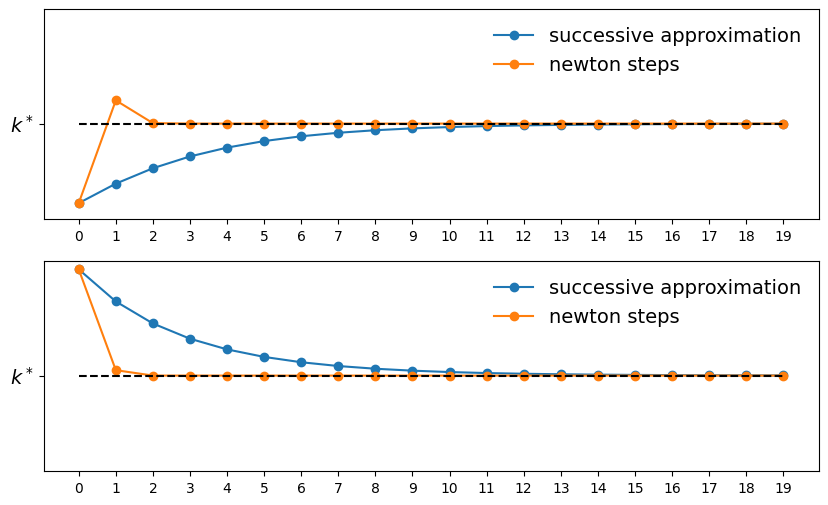
_images/dd2e216f11e6834447ec3732042142c2775ee89543ed2eb128124ba2819b9aea.png

We can see that Newton’s method converges faster than successive approximation.

7.3. Root-Finding in one dimension #

In the previous section we computed fixed points.

In fact Newton’s method is more commonly associated with the problem of finding zeros of functions.

Let’s discuss this “root-finding” problem and then show how it is connected to the problem of finding fixed points.

7.3.1. Newton’s method for zeros#

Let’s suppose we want to find an $x$ such that $f (x) = 0$ for some smooth function $f$ mapping real numbers to real numbers.

Suppose we have a guess $x_{0}$ and we want to update it to a new point $x_{1}$ .

As a first step, we take the first-order approximation of $f$ around $x_{0}$ :

\hat{f} (x) \approx f (x_{0}) + f^{'} (x_{0}) (x - x_{0})

Now we solve for the zero of $\hat{f}$ .

In particular, we set $\hat{f} (x_{1}) = 0$ and solve for $x_{1}$ to get

x_{1} = x_{0} - \frac{f (x_{0})}{f^{'} (x_{0})}, x_{0} given

Generalizing the formula above, for one-dimensional zero-finding problems, Newton’s method iterates on

(7.5)#

x_{t + 1} = x_{t} - \frac{f (x_{t})}{f^{'} (x_{t})}, x_{0} given

The following code implements the iteration (7.5)

def newton(f, x_0, tol=1e-7, max_iter=100_000):
    x = x_0
    Df = jax.grad(f)

    # Implement the zero-finding formula
    @jax.jit
    def q(x):
        return x - f(x) / Df(x)

    error = tol + 1
    n = 0
    while error > tol:
        n += 1
        if n > max_iter:
            raise Exception("Max iteration reached without convergence")
        y = q(x)
        error = jnp.abs(x - y)
        x = y
        print(f"iteration {n}, error = {error:.5f}")
    return x.item()

Numerous libraries implement Newton’s method in one dimension, including SciPy, so the code is just for illustrative purposes.

(That said, when we want to apply Newton’s method using techniques such as automatic differentiation or GPU acceleration, it will be helpful to know how to implement Newton’s method ourselves.)

7.3.2. Application to finding fixed points#

Now consider again the Solow fixed-point calculation, where we solve for $k$ satisfying $g (k) = k$ .

We can convert to this to a zero-finding problem by setting $f (x) := g (x) - x$ .

Any zero of $f$ is clearly a fixed point of $g$ .

Let’s apply this idea to the Solow problem

params = create_solow_params()
k_star_approx_newton = newton(f = lambda x: g(x, params) - x, x_0=0.8)

iteration 1, error = 1.27209
iteration 2, error = 0.28180
iteration 3, error = 0.00561
iteration 4, error = 0.00000
iteration 5, error = 0.00000

k_star_approx_newton

1.7846741842265788

The result confirms convergence we saw in the graphs above: a very accurate result is reached with only 5 iterations.

7.4. Multivariate Newton’s method #

In this section, we introduce a two-good problem, present a visualization of the problem, and solve for the equilibrium of the two-good market using both a zero finder in SciPy and Newton’s method.

We then expand the idea to a larger market with 5,000 goods and compare the performance of the two methods again.

We will see a significant performance gain when using Newton’s method.

7.4.1. A two-goods market equilibrium#

Let’s start by computing the market equilibrium of a two-good problem.

We consider a market for two related products, good 0 and good 1, with price vector $p = (p_{0}, p_{1})$

Supply of good $i$ at price $p$ ,

q_{i}^{s} (p) = b_{i} \sqrt{p_{i}}

Demand of good $i$ at price $p$ is,

q_{i}^{d} (p) = \exp (- (a_{i 0} p_{0} + a_{i 1} p_{1})) + c_{i}

Here $c_{i}$ , $b_{i}$ and $a_{i j}$ are parameters.

For example, the two goods might be computer components that are typically used together, in which case they are complements. Hence demand depends on the price of both components.

The excess demand function is,

e_{i} (p) = q_{i}^{d} (p) - q_{i}^{s} (p), i = 0, 1

An equilibrium price vector $p^{*}$ satisfies $e_{i} (p^{*}) = 0$ .

We set

\begin{array}{r} A = [\begin{array}{c} a_{00} & a_{01} \\ a_{10} & a_{11} \end{array}], b = [\begin{array}{c} b_{0} \\ b_{1} \end{array}] and c = [\begin{array}{c} c_{0} \\ c_{1} \end{array}] \end{array}

for this particular question.

7.4.1.1. A graphical exploration#

Since our problem is only two-dimensional, we can use graphical analysis to visualize and help understand the problem.

Our first step is to define the excess demand function

\begin{array}{r} e (p) = [\begin{array}{c} e_{0} (p) \\ e_{1} (p) \end{array}] \end{array}

The function below calculates the excess demand for given parameters

@jax.jit
def e(p, A, b, c):
    return jnp.exp(-A @ p) + c - b * jnp.sqrt(p)

Our default parameter values will be

\begin{array}{r} A = [\begin{array}{c} 0.5 & 0.4 \\ 0.8 & 0.2 \end{array}], b = [\begin{array}{c} 1 \\ 1 \end{array}] and c = [\begin{array}{c} 1 \\ 1 \end{array}] \end{array}

A = jnp.array([[0.5, 0.4], [0.8, 0.2]])
b = jnp.ones(2)
c = jnp.ones(2)

At a price level of $p = (1, 0.5)$ , the excess demand is

p = jnp.array([1, 0.5])
ex_demand = e(p, A, b, c)

print(
    f"The excess demand for good 0 is {ex_demand[0]:.3f} \n"
    f"The excess demand for good 1 is {ex_demand[1]:.3f}"
)

The excess demand for good 0 is 0.497 
The excess demand for good 1 is 0.699

To increase the efficiency of computation, we will use the power of vectorization using jax.vmap. This is much faster than the python loops.

# Create vectorization on the first axis of p.
e_vectorized_p_1 = jax.vmap(e, in_axes=(0, None, None, None))

# Create vectorization on the second axis of p.
e_vectorized = jax.vmap(e_vectorized_p_1, in_axes=(0, None, None, None))

Next we plot the two functions $e_{0}$ and $e_{1}$ on a grid of $(p_{0}, p_{1})$ values, using contour surfaces and lines.

We will use the following function to build the contour plots

def plot_excess_demand(ax, good=0, grid_size=100, grid_max=4, surface=True):
    p_grid = jnp.linspace(0, grid_max, grid_size)

    # Create meshgrid for all combinations of p_1 and p_2
    P1, P2 = jnp.meshgrid(p_grid, p_grid, indexing="ij")

    # Stack to create array of shape (grid_size, grid_size, 2)
    P = jnp.stack([P1, P2], axis=-1)

    # Compute all values at once using vectorized function
    z_full = e_vectorized(P, A, b, c)
    z = z_full[:, :, good]

    if surface:
        cs1 = ax.contourf(p_grid, p_grid, z.T, alpha=0.5)
        plt.colorbar(cs1, ax=ax, format="%.6f")

    ctr1 = ax.contour(p_grid, p_grid, z.T, levels=[0.0])
    ax.set_xlabel("$p_0$")
    ax.set_ylabel("$p_1$")
    ax.set_title(f"Excess demand for good {good}")
    plt.clabel(ctr1, inline=1, fontsize=13)

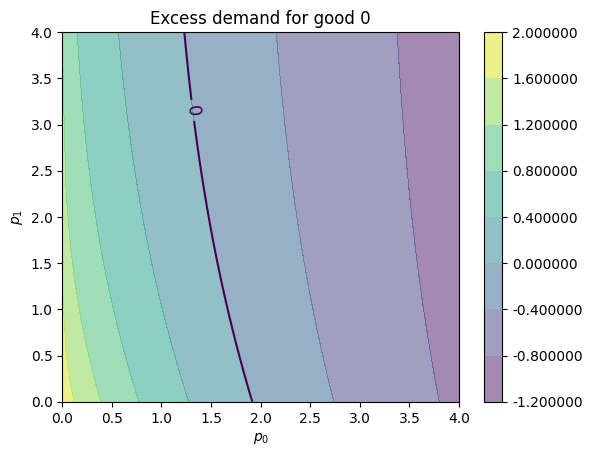
Here’s our plot of $e_{0}$ :

fig, ax = plt.subplots()
plot_excess_demand(ax, good=0)
plt.show()

_images/241a702cd537d2eae4fecfbbdf6e865616cd4d3767da1cb276ca9af1f722382d.png

Here’s our plot of $e_{1}$ :

fig, ax = plt.subplots()
plot_excess_demand(ax, good=1)
plt.show()

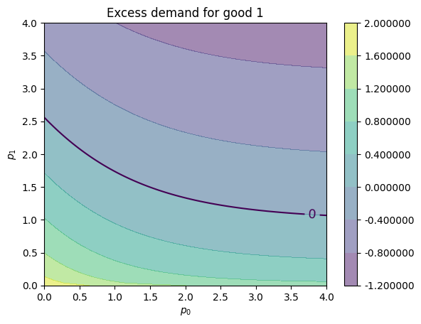
_images/429010ebb9b1aaa33f4d4733bd5ac85de8309ec713fb8b81192889556962b5dc.png

We see the black contour line of zero, which tells us when $e_{i} (p) = 0$ .

For a price vector $p$ such that $e_{i} (p) = 0$ we know that good $i$ is in equilibrium (demand equals supply).

If these two contour lines cross at some price vector $p^{*}$ , then $p^{*}$ is an equilibrium price vector.

fig, ax = plt.subplots(figsize=(10, 5.7))
for good in (0, 1):
    plot_excess_demand(ax, good=good, surface=False)
plt.show()

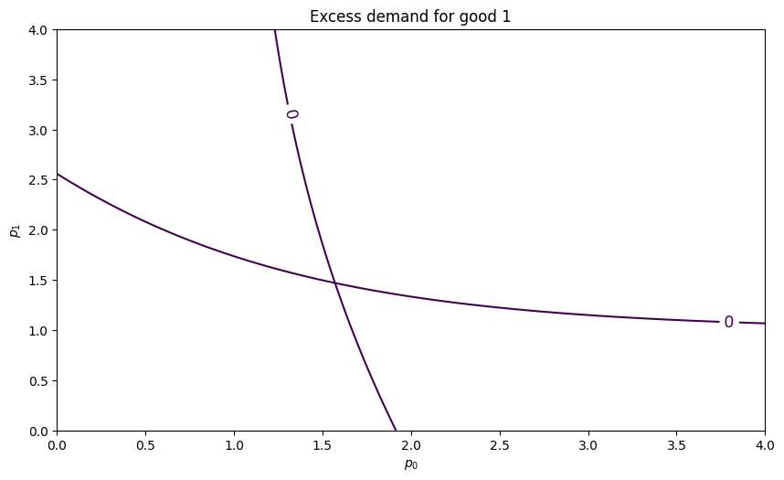
_images/c59a036425c6b87d9c5db9606122e5a5fe805832196526fdb0ab8b8ffeecf6cd.png

It seems there is an equilibrium close to $p = (1.6, 1.5)$ .

7.4.1.2. Using a multidimensional root finder#

To solve for $p^{*}$ more precisely, we use a zero-finding algorithm from scipy.optimize.

We supply $p = (1, 1)$ as our initial guess.

init_p = jnp.ones(2)

This uses the modified Powell method to find the zero

%%time
solution = root(lambda p: e(p, A, b, c), init_p, method="hybr")

CPU times: user 8.29 ms, sys: 1.49 ms, total: 9.77 ms
Wall time: 5.39 ms

Here’s the resulting value:

p = solution.x
p

array([1.57080182, 1.46928838])

This looks close to our guess from observing the figure. We can plug it back into $e$ to test that $e (p) \approx 0$ :

e_p = jnp.max(jnp.abs(e(p, A, b, c)))
e_p.item()

2.0383694732117874e-13

This is indeed a very small error.

7.4.1.3. Adding gradient information#

In many cases, for zero-finding algorithms applied to smooth functions, supplying the Jacobian of the function leads to better convergence properties.

Here, we manually calculate the elements of the Jacobian

\begin{array}{r} J (p) = [\begin{array}{c} \frac{\partial e_{0}}{\partial p_{0}} (p) & \frac{\partial e_{0}}{\partial p_{1}} (p) \\ \frac{\partial e_{1}}{\partial p_{0}} (p) & \frac{\partial e_{1}}{\partial p_{1}} (p) \end{array}] \end{array}

def jacobian_e(p, A, b, c):
    p_0, p_1 = p
    a_00, a_01 = A[0, :]
    a_10, a_11 = A[1, :]
    j_00 = -a_00 * jnp.exp(-a_00 * p_0) - (b[0] / 2) * p_0 ** (-1 / 2)
    j_01 = -a_01 * jnp.exp(-a_01 * p_1)
    j_10 = -a_10 * jnp.exp(-a_10 * p_0)
    j_11 = -a_11 * jnp.exp(-a_11 * p_1) - (b[1] / 2) * p_1 ** (-1 / 2)
    J = [[j_00, j_01], [j_10, j_11]]
    return jnp.array(J)

%%time
solution = root(
    lambda p: e(p, A, b, c),
    init_p,
    jac = lambda p: jacobian_e(p, A, b, c),
    method="hybr"
)

CPU times: user 280 ms, sys: 9.32 ms, total: 290 ms
Wall time: 389 ms

Now the solution is even more accurate (although, in this low-dimensional problem, the difference is quite small):

p = solution.x
e_p = jnp.max(jnp.abs(e(p, A, b, c)))
e_p.item()

1.3322676295501878e-15

7.4.1.4. Using Newton’s method#

Now let’s use Newton’s method to compute the equilibrium price using the multivariate version of Newton’s method

(7.6)#

p_{n + 1} = p_{n} - J_{e} (p_{n})^{- 1} e (p_{n})

This is a multivariate version of (7.5)

(Here $J_{e} (p_{n})$ is the Jacobian of $e$ evaluated at $p_{n}$ .)

The iteration starts from some initial guess of the price vector $p_{0}$ .

Here, instead of coding Jacobian by hand, we use the jacobian() function in the jax library to auto-differentiate and calculate the Jacobian.

With only slight modification, we can generalize our previous attempt to multidimensional problems

def newton(f, x_0, tol=1e-5, max_iter=10):
    x = x_0
    f_jac = jax.jacobian(f)

    @jax.jit
    def q(x):
        return x - jnp.linalg.solve(f_jac(x), f(x))

    error = tol + 1
    n = 0
    while error > tol:
        n += 1
        if n > max_iter:
            raise Exception("Max iteration reached without convergence")
        y = q(x)
        if any(jnp.isnan(y)):
            raise Exception("Solution not found with NaN generated")
        error = jnp.linalg.norm(x - y)
        x = y
        print(f"iteration {n}, error = {error:.5f}")
    print("\n" + f"Result = {x} \n")
    return x

We find the algorithm terminates in 4 steps

%%time
p = newton(lambda p: e(p, A, b, c), init_p)

iteration 1, error = 0.62515
iteration 2, error = 0.11152
iteration 3, error = 0.00258
iteration 4, error = 0.00000

Result = [1.57080182 1.46928838] 

CPU times: user 363 ms, sys: 24.5 ms, total: 388 ms
Wall time: 461 ms

e_p = jnp.max(jnp.abs(e(p, A, b, c)))
e_p.item()

1.4632739464559563e-13

The result is very accurate.

With the larger overhead, the speed is not better than the optimized scipy function.

7.4.2. A high-dimensional problem#

Our next step is to investigate a large market with 3,000 goods.

The excess demand function is essentially the same, but now the matrix $A$ is $3000 \times 3000$ and the parameter vectors $b$ and $c$ are $3000 \times 1$ .

dim = 3000

# Create JAX random key
key = jax.random.PRNGKey(123)

# Create a random matrix A and normalize the columns to sum to one
A = jax.random.uniform(key, (dim, dim))
s = jnp.sum(A, axis=0)
A = A / s

# Set up b and c
b = jnp.ones(dim)
c = jnp.ones(dim)

Here’s our initial condition

init_p = jnp.ones(dim)

%%time
p = newton(lambda p: e(p, A, b, c), init_p)

iteration 1, error = 23.22268

iteration 2, error = 3.94538

iteration 3, error = 0.08500

iteration 4, error = 0.00004

iteration 5, error = 0.00000

Result = [1.50795569 1.50865411 1.50343775 ... 1.48769903 1.48916887 1.49997787] 

CPU times: user 6.96 s, sys: 2.22 s, total: 9.18 s
Wall time: 8.75 s

e_p = jnp.max(jnp.abs(e(p, A, b, c)))
e_p.item()

4.440892098500626e-16

With the same tolerance, we compare the runtime and accuracy of Newton’s method to SciPy’s root function

%%time
solution = root(
    lambda p: e(p, A, b, c),
    init_p,
    jac = lambda p: jax.jacobian(e)(p, A, b, c),
    method="hybr",
    tol=1e-5,
)

CPU times: user 33.1 s, sys: 27.8 ms, total: 33.1 s
Wall time: 33.6 s

p = solution.x
e_p = jnp.max(jnp.abs(e(p, A, b, c)))
e_p.item()

9.006137220435306e-07

7.5. Exercises #

Exercise 7.1

Consider a three-dimensional extension of the Solow fixed point problem with

\begin{array}{r} A = [\begin{array}{c} 2 & 3 & 3 \\ 2 & 4 & 2 \\ 1 & 5 & 1 \end{array}], s = 0.2, α = 0.5, δ = 0.8 \end{array}

As before the law of motion is

k_{t + 1} = g (k_{t}) where g (k) := s A k^{α} + (1 - δ) k

However, $k_{t}$ is now a $3 \times 1$ vector.

Solve for the fixed point using Newton’s method with the following initial values:

\begin{array}{r} \begin{aligned} k 1_{0} & = (1, 1, 1) \\ k 2_{0} & = (3, 5, 5) \\ k 3_{0} & = (50, 50, 50) \end{aligned} \end{array}

Hint

The computation of the fixed point is equivalent to computing $k^{*}$ such that $g (k^{*}) - k^{*} = 0$ .
If you are unsure about your solution, you can start with the solved example:

\begin{array}{r} A = [\begin{array}{c} 2 & 0 & 0 \\ 0 & 2 & 0 \\ 0 & 0 & 2 \end{array}] \end{array}

with $s = 0.3$ , $α = 0.3$ , and $δ = 0.4$ and starting value:

k_{0} = (1, 1, 1)

The result should converge to the analytical solution.

Solution to Exercise 7.1

Let’s first define the parameters for this problem

A = jnp.array([[2.0, 3.0, 3.0], [2.0, 4.0, 2.0], [1.0, 5.0, 1.0]])

s = 0.2
α = 0.5
δ = 0.8

initLs = [jnp.ones(3), jnp.array([3.0, 5.0, 5.0]), jnp.repeat(50.0, 3)]

Then define the multivariate version of the formula for the (7.1)

@jax.jit
def multivariate_solow(k, A=A, s=s, α=α, δ=δ):
    return s * jnp.dot(A, k**α) + (1 - δ) * k

Let’s run through each starting value and see the output

attempt = 1
for init in initLs:
    print(f'Attempt {attempt}: Starting value is {init} \n')
    %time k = newton(lambda k: multivariate_solow(k) - k, \
                    init)
    print('-'*64)
    attempt += 1

Attempt 1: Starting value is [1. 1. 1.]

iteration 1, error = 50.49630
iteration 2, error = 41.10937
iteration 3, error = 4.29413
iteration 4, error = 0.38543
iteration 5, error = 0.00544
iteration 6, error = 0.00000

Result = [3.84058108 3.87071771 3.41091933] 

CPU times: user 257 ms, sys: 24.6 ms, total: 281 ms
Wall time: 340 ms
----------------------------------------------------------------
Attempt 2: Starting value is [3. 5. 5.] 

iteration 1, error = 2.07011
iteration 2, error = 0.12642
iteration 3, error = 0.00060
iteration 4, error = 0.00000

Result = [3.84058108 3.87071771 3.41091933] 

CPU times: user 113 ms, sys: 6.47 ms, total: 120 ms
Wall time: 132 ms
----------------------------------------------------------------
Attempt 3: Starting value is [50. 50. 50.]

iteration 1, error = 73.00943
iteration 2, error = 6.49379
iteration 3, error = 0.68070
iteration 4, error = 0.01620
iteration 5, error = 0.00001
iteration 6, error = 0.00000

Result = [3.84058108 3.87071771 3.41091933] 

CPU times: user 261 ms, sys: 18.2 ms, total: 279 ms
Wall time: 316 ms
----------------------------------------------------------------

We find that the results are invariant to the starting values given the well-defined property of this question.

But the number of iterations it takes to converge is dependent on the starting values.

Let’s substitute the output back into the formula to check our last result

multivariate_solow(k) - k

Array([0., 0., 0.], dtype=float64)

Note the error is very small.

We can also test our results on the known solution

A = jnp.array([[2.0, 0.0, 0.0],
               [0.0, 2.0, 0.0],
               [0.0, 0.0, 2.0]])

s = 0.3
α = 0.3
δ = 0.4

init = jnp.repeat(1.0, 3)


%time k = newton(lambda k: multivariate_solow(k, A=A, s=s, α=α, δ=δ) - k, \
                 init)

iteration 1, error = 1.57459
iteration 2, error = 0.21345
iteration 3, error = 0.00205
iteration 4, error = 0.00000

Result = [1.78467418 1.78467418 1.78467418] 

CPU times: user 232 ms, sys: 23.7 ms, total: 256 ms
Wall time: 283 ms

The result is very close to the ground truth but still slightly different.

%time k = newton(lambda k: multivariate_solow(k, A=A, s=s, α=α, δ=δ) - k, \
                 init,\
                 tol=1e-7)

iteration 1, error = 1.57459
iteration 2, error = 0.21345
iteration 3, error = 0.00205
iteration 4, error = 0.00000
iteration 5, error = 0.00000

Result = [1.78467418 1.78467418 1.78467418] 

CPU times: user 224 ms, sys: 16.1 ms, total: 240 ms
Wall time: 265 ms

We can see it steps towards a more accurate solution.

Exercise 7.2

In this exercise, let’s try different initial values and check how Newton’s method responds to different starting points.

Let’s define a three-good problem with the following default values:

\begin{array}{r} A = [\begin{array}{c} 0.2 & 0.1 & 0.7 \\ 0.3 & 0.2 & 0.5 \\ 0.1 & 0.8 & 0.1 \end{array}], b = [\begin{array}{c} 1 \\ 1 \\ 1 \end{array}] and c = [\begin{array}{c} 1 \\ 1 \\ 1 \end{array}] \end{array}

For this exercise, use the following extreme price vectors as initial values:

\begin{array}{r} \begin{aligned} p 1_{0} & = (5, 5, 5) \\ p 2_{0} & = (1, 1, 1) \\ p 3_{0} & = (4.5, 0.1, 4) \end{aligned} \end{array}

Set the tolerance to $1 e - 15$ for more accurate output.

Solution to Exercise 7.2

Define parameters and initial values

A = jnp.array([[0.2, 0.1, 0.7], [0.3, 0.2, 0.5], [0.1, 0.8, 0.1]])
b = jnp.array([1.0, 1.0, 1.0])
c = jnp.array([1.0, 1.0, 1.0])

initLs = [jnp.repeat(5.0, 3), jnp.ones(3), jnp.array([4.5, 0.1, 4.0])]

Let’s run through each initial guess and check the output

attempt = 1
for init in initLs:
    print(f'Attempt {attempt}: Starting value is {init} \n')
    %time p = newton(lambda p: e(p, A, b, c), \
                init, \
                tol=1e-15, \
                max_iter=15)
    print('-'*64)
    attempt += 1

Attempt 1: Starting value is [5. 5. 5.]

iteration 1, error = 9.24381

---------------------------------------------------------------------------
Exception                                 Traceback (most recent call last)
<timed exec> in <module>

/tmp/ipython-input-1446471363.py in newton(f, x_0, tol, max_iter)
     15         y = q(x)
     16         if any(jnp.isnan(y)):
---> 17             raise Exception("Solution not found with NaN generated")
     18         error = jnp.linalg.norm(x - y)
     19         x = y

Exception: Solution not found with NaN generated

----------------------------------------------------------------
Attempt 2: Starting value is [1. 1. 1.] 

iteration 1, error = 0.73419
iteration 2, error = 0.12472
iteration 3, error = 0.00269
iteration 4, error = 0.00000
iteration 5, error = 0.00000
iteration 6, error = 0.00000

Result = [1.49744442 1.49744442 1.49744442] 

CPU times: user 102 ms, sys: 11.7 ms, total: 114 ms
Wall time: 125 ms
----------------------------------------------------------------
Attempt 3: Starting value is [4.5 0.1 4. ]

iteration 1, error = 4.89202
iteration 2, error = 1.21206
iteration 3, error = 0.69421
iteration 4, error = 0.16895
iteration 5, error = 0.00521
iteration 6, error = 0.00000
iteration 7, error = 0.00000
iteration 8, error = 0.00000

Result = [1.49744442 1.49744442 1.49744442] 

CPU times: user 113 ms, sys: 6.43 ms, total: 119 ms
Wall time: 126 ms
----------------------------------------------------------------

We can see that Newton’s method may fail for some starting values.

Sometimes it may take a few initial guesses to achieve convergence.

Substitute the result back to the formula to check our result

e(p, A, b, c)

Array([0., 0., 0.], dtype=float64)

We can see the result is very accurate.

7. Using Newton’s Method to Solve Economic Models#

7.1. Overview#

7.2. Fixed point computation using Newton’s method#

7.2.1. The Solow model#

7.2.2. Implementation#

7.2.2.1. Successive approximation#

7.2.2.2. Newton’s method#

7.3. Root-Finding in one dimension#

7.3.1. Newton’s method for zeros#

7.3.2. Application to finding fixed points#

7.4. Multivariate Newton’s method#

7.4.1. A two-goods market equilibrium#

7.4.1.1. A graphical exploration#

7.4.1.2. Using a multidimensional root finder#

7.4.1.3. Adding gradient information#

7.4.1.4. Using Newton’s method#

7.4.2. A high-dimensional problem#

7.5. Exercises#

7. Using Newton’s Method to Solve Economic Models #

7.1. Overview #

7.2. Fixed point computation using Newton’s method #

7.3. Root-Finding in one dimension #

7.4. Multivariate Newton’s method #

7.5. Exercises #