23. Heterogeneous Beliefs and Financial Markets#

23.1. Overview#

A likelihood ratio process lies behind Lawrence Blume and David Easley’s answer to their question ‘‘If you’re so smart, why aren’t you rich?’’ [Blume and Easley, 2006].

Blume and Easley constructed formal models to study how differences of opinions about probabilities governing risky income processes would influence outcomes and be reflected in prices of stocks, bonds, and insurance policies that individuals use to share and hedge risks.

Here we’ll provide an example that illustrates basic components of Blume and Easley’s analysis.

We’ll focus only on their analysis of an environment with complete markets in which trades in all conceivable risky securities are possible.

We’ll study two alternative arrangements:

• perfect socialism in which individuals surrender their endowments of consumption goods each period to a central planner who then dictatorially allocates those goods

• a decentralized system of competitive markets in which selfish price-taking individuals voluntarily trade with each other in competitive markets

The fundamental theorems of welfare economics will apply and assure us that these two arrangements end up producing exactly the same allocation of consumption goods to individuals provided that the social planner assigns an appropriate set of Pareto weights.

Let’s start by importing some Python tools.

import matplotlib.pyplot as plt
import numpy as np
from numba import vectorize, jit
from math import gamma
from scipy.integrate import quad
from scipy.optimize import brentq, minimize_scalar
import pandas as pd
from IPython.display import display, Math
import quantecon as qe

23.2. Review: Likelihood Ratio Processes#

We’ll begin by reminding ourselves definitions and properties of likelihood ratio processes.

A nonnegative random variable $W$ has one of two probability density functions, either $f$ or $g$.

Before the beginning of time, nature once and for all decides whether she will draw a sequence of IID draws from either $f$ or $g$.

We will sometimes let $q$ be the density that nature chose once and for all, so that $q$ is either $f$ or $g$, permanently.

Nature knows which density it permanently draws from, but we the observers do not.

We know both $f$ and $g$ but we don’t know which density nature chose.

But we want to know.

To do that, we use observations.

We observe a sequence $\{w_t{\}}_{t=1}^T$ of $T$ IID draws that we know came from either $f$ or $g$.

We want to use these observations to infer whether nature chose $f$ or $g$.

A likelihood ratio process is a useful tool for this task.

To begin, we define a key component of a likelihood ratio process, namely, the time $t$ likelihood ratio as the random variable

We assume that $f$ and $g$ both put positive probabilities on the same intervals of possible realizations of the random variable $W$.

That means that under the $g$ density, $\ell (w_t)=\frac{f\left(w_t\right)}{g\left(w_t\right)}$ is a nonnegative random variable with mean $1$.

A likelihood ratio process for sequence ${\left\{w_t\right\}}_{t=1}^{\mathrm{\infty }}$ is defined as

where $w^t=\{w_1,\dots ,w_t\}$ is a history of observations up to and including time $t$.

Sometimes for shorthand we’ll write $L_t=L(w^t)$.

Notice that the likelihood process satisfies the recursion

The likelihood ratio and its logarithm are key tools for making inferences using a classic frequentist approach due to Neyman and Pearson [Neyman and Pearson, 1933].

To help us appreciate how things work, the following Python code evaluates $f$ and $g$ as two different Beta distributions, then computes and simulates an associated likelihood ratio process by generating a sequence $w^t$ from one of the two probability distributions, for example, a sequence of IID draws from $g$.

# Parameters in the two Beta distributions.
F_a, F_b = 1, 1
G_a, G_b = 3, 1.2

@vectorize
def p(x, a, b):
    r = gamma(a + b) / (gamma(a) * gamma(b))
    return r * x** (a-1) * (1 - x) ** (b-1)

# The two density functions.
f = jit(lambda x: p(x, F_a, F_b))
g = jit(lambda x: p(x, G_a, G_b))

@jit
def simulate(a, b, T=50, N=500):
    '''
    Generate N sets of T observations of the likelihood ratio,
    return as N x T matrix.
    '''

    l_arr = np.empty((N, T))

    for i in range(N):
        for j in range(T):
            w = np.random.beta(a, b)
            l_arr[i, j] = f(w) / g(w)

    return l_arr

23.3. Blume and Easley’s Setting#

Let the random variable $s_t\in (0,1)$ at time $t=0,1,2,\dots$ be distributed according to the same Beta distribution with parameters $\theta =\{{\theta }_1,{\theta }_2\}$.

We’ll denote this probability density as

Below, we’ll often just write $\pi (s_t)$ instead of $\pi (s_t|\theta )$ to save space.

Let $s_t\equiv y_t^1$ be the endowment of a nonstorable consumption good that a person we’ll call “agent 1” receives at time $t$.

Let a history $s^t=[s_t,s_{t-1},\dots ,s_0]$ be a sequence of i.i.d. random variables with joint distribution

So in our example, the history $s^t$ is a comprehensive record of agent $1$’s endowments of the consumption good from time $0$ up to time $t$.

If agent $1$ were to live on an island by himself, agent $1$’s consumption $c^1(s_t)$ at time $t$ is

But in our model, agent 1 is not alone.

23.4. Nature and Agents’ Beliefs#

Nature draws i.i.d. sequences $\{s_t{\}}_{t=0}^{\mathrm{\infty }}$ from ${\pi }_t(s^t)$.

• so $\pi$ without a superscript is nature’s model

• but in addition to nature, there are other entities inside our model – artificial people that we call “agents”

• each agent has a sequence of probability distributions over $s^t$ for $t=0,\dots$

• agent $i$ thinks that nature draws i.i.d. sequences $\{s_t{\}}_{t=0}^{\mathrm{\infty }}$ from $\{{\pi }_t^i(s^t){\}}_{t=0}^{\mathrm{\infty }}$

  • agent $i$ is mistaken unless ${\pi }_t^i(s^t)={\pi }_t(s^t)$

There are two agents named $i=1$ and $i=2$.

At time $t$, agent $1$ receives an endowment

of a nonstorable consumption good, while agent $2$ receives an endowment of

The aggregate endowment of the consumption good is

at each date $t\ge 0$.

At date $t$ agent $i$ consumes $c_t^i(s^t)$ of the good.

A (non wasteful) feasible allocation of the aggregate endowment of $1$ each period satisfies

23.5. A Socialist Risk-Sharing Arrangement#

In order to share risks, a benevolent social planner dictates a history-dependent consumption allocation that takes the form of a sequence of functions

that satisfy

for all $s^t$ for all $t\ge 0$.

To design a socially optimal allocation, the social planner wants to know what agent $1$ believes about the endowment sequence and how they feel about bearing risks.

As for the endowment sequences, agent $i$ believes that nature draws i.i.d. sequences from joint densities

As for attitudes toward bearing risks, agent $i$ has a one-period utility function

with marginal utility of consumption in period $i$

Putting its beliefs about its random endowment sequence and its attitudes toward bearing risks together, agent $i$ has intertemporal utility function

where $\delta \in (0,1)$ is an intertemporal discount factor, and $u(\cdot )$ is a strictly increasing, concave one-period utility function.

23.6. Social Planner’s Allocation Problem#

The benevolent dictator has all the information it requires to choose a consumption allocation that maximizes the social welfare criterion

where $\lambda \in [0,1]$ is a Pareto weight that tells how much the planner likes agent $1$ and $1-\lambda$ is a Pareto weight that tells how much the social planner likes agent $2$.

Setting $\lambda =.5$ expresses ‘‘egalitarian’’ social preferences.

Notice how social welfare criterion (23.3) takes into account both agents’ preferences as represented by formula (23.2).

This means that the social planner knows and respects

• each agent’s one period utility function $u(\cdot )=\ln (\cdot )$

• each agent $i$’s probability model $\{{\pi }_t^i(s^t){\}}_{t=0}^{\mathrm{\infty }}$

Consequently, we anticipate that these objects will appear in the social planner’s rule for allocating the aggregate endowment each period.

First-order necessary conditions for maximizing welfare criterion (23.3) subject to the feasibility constraint (23.1) are

which can be rearranged to become

where

is the likelihood ratio of agent 1’s joint density to agent 2’s joint density.

Using

we can rewrite allocation rule (23.4) as

or

which implies that the social planner’s allocation rule is

If we define a temporary or continuation Pareto weight process as

then we can represent the social planner’s allocation rule as

23.7. If You’re So Smart, $\dots$#

Let’s compute some values of limiting allocations (23.5) for some interesting possible limiting values of the likelihood ratio process $l_t(s^t)$:

• In the above case, both agents are equally smart (or equally not smart) and the consumption allocation stays put at a $\lambda ,1-\lambda$ split between the two agents.

• In the above case, agent 2 is ‘‘smarter’’ than agent 1, and agent 1’s share of the aggregate endowment converges to zero.

• In the above case, agent 1 is smarter than agent 2, and agent 1’s share of the aggregate endowment converges to 1.

Soon we’ll do some simulations that will shed further light on possible outcomes.

But before we do that, let’s take a detour and study some “shadow prices” for the social planning problem that can readily be converted to “equilibrium prices” for a competitive equilibrium.

Doing this will allow us to connect our analysis with an argument of [Alchian, 1950] and [Friedman, 1953] that competitive market processes can make prices of risky assets better reflect realistic probability assessments.

23.8. Competitive Equilibrium Prices#

Two fundamental welfare theorems for general equilibrium models lead us to anticipate that there is a connection between the allocation that solves the social planning problem we have been studying and the allocation in a competitive equilibrium with complete markets in history-contingent commodities.

Such a connection prevails for our model.

We’ll sketch it now.

In a competitive equilibrium, there is no social planner that dictatorially collects everybody’s endowments and then reallocates them.

Instead, there is a comprehensive centralized market that meets at one point in time.

There are prices at which price-taking agents can buy or sell whatever goods that they want.

Trade is multilateral in the sense that that there is a “Walrasian auctioneer” who lives outside the model and whose job is to verify that each agent’s budget constraint is satisfied.

That budget constraint involves the total value of the agent’s endowment stream and the total value of its consumption stream.

These values are computed at price vectors that the agents take as given – they are “price-takers” who assume that they can buy or sell whatever quantities that they want at those prices.

Suppose that at time $-1$, before time $0$ starts, agent $i$ can purchase one unit $c_t(s^t)$ of consumption at time $t$ after history $s^t$ at price $p_t(s^t)$.

Notice that there is (very long) vector of prices.

• there is one price $p_t(s^t)$ for each history $s^t$ at every date $t=0,1,\dots ,$.

• so there are as many prices as there are histories and dates.

These prices determined at time $-1$ before the economy starts.

The market meets once at time $-1$.

At times $t=0,1,2,\dots$ trades made at time $-1$ are executed.

• in the background, there is an “enforcement” procedure that forces agents to carry out the exchanges or “deliveries” that they agreed to at time $-1$.

We want to study how agents’ beliefs influence equilibrium prices.

Agent $i$ faces a single intertemporal budget constraint

According to budget constraint (23.6), trade is multilateral in the following sense

• we can imagine that agent $i$ first sells his random endowment stream $\{y_t^i(s^t)\}$ and then uses the proceeds (i.e., his “wealth”) to purchase a random consumption stream $\{c_t^i(s^t)\}$.

Agent $i$ puts a Lagrange multiplier ${\mu }_i$ on (23.6) and once-and-for-all chooses a consumption plan $\{c_t^i(s^t){\}}_{t=0}^{\mathrm{\infty }}$ to maximize criterion (23.2) subject to budget constraint (23.6).

This means that the agent $i$ chooses many objects, namely, $c_t^i(s^t)$ for all $s^t$ for $t=0,1,2,\dots$.

For convenience, let’s remind ourselves of criterion $V^i$ defined in (23.2):

First-order necessary conditions for maximizing objective $V^i$ defined in (23.2) with respect to $c_t^i(s^t)$ are

which we can rearrange to obtain

for $i=1,2$.

If we divide equation (23.7) for agent $1$ by the appropriate version of equation (23.7) for agent 2, use $c_t^2(s^t)=1-c_t^1(s^t)$, and do some algebra, we’ll obtain

We now engage in an extended “guess-and-verify” exercise that involves matching objects in our competitive equilibrium with objects in our social planning problem.

• we’ll match consumption allocations in the planning problem with equilibrium consumption allocations in the competitive equilibrium

• we’ll match “shadow” prices in the planning problem with competitive equilibrium prices.

Notice that if we set ${\mu }_1=1-\lambda$ and ${\mu }_2=\lambda$, then formula (23.8) agrees with formula (23.5).

• doing this amounts to choosing a numeraire or normalization for the price system $\{p_t(s^t){\}}_{t=0}^{\mathrm{\infty }}$

If we substitute formula (23.8) for $c_t^1(s^t)$ into formula (23.7) and rearrange, we obtain

or

According to formula (23.9), we have the following possible limiting cases:

• when $l_{\mathrm{\infty }}=0$, $c_{\mathrm{\infty }}^1=0$ and tails of competitive equilibrium prices reflect agent $2$’s probability model ${\pi }_t^2(s^t)$ according to $p_t(s^t)\propto {\delta }^t{\pi }_t^2(s^t)$

• when $l_{\mathrm{\infty }}=\mathrm{\infty }$, $c_{\mathrm{\infty }}^1=1$ and tails of competitive equilibrium prices reflect agent $1$’s probability model ${\pi }_t^1(s^t)$ according to $p_t(s^t)\propto {\delta }^t{\pi }_t^1(s^t)$

• for small $t$’s, competitive equilibrium prices reflect both agents’ probability models.

23.9. Simulations#

Now let’s implement some simulations when agent $1$ believes marginal density

and agent $2$ believes marginal density

where $f$ and $g$ are Beta distributions like ones that we used in earlier sections of this lecture.

Meanwhile, we’ll assume that nature believes a marginal density

where $h(s_t)$ is perhaps a mixture of $f$ and $g$.

First, we write a function to compute the likelihood ratio process

def compute_likelihood_ratios(sequences, f, g):
    """Compute likelihood ratios and cumulative products."""
    l_ratios = f(sequences) / g(sequences)
    L_cumulative = np.cumprod(l_ratios, axis=1)
    return l_ratios, L_cumulative

Let’s compute the Kullback–Leibler discrepancies by quadrature integration.

def compute_KL(f, g):
    """
    Compute KL divergence KL(f, g)
    """
    integrand = lambda w: f(w) * np.log(f(w) / g(w))
    val, _ = quad(integrand, 1e-5, 1-1e-5)
    return val

We also create a helper function to compute KL divergence with respect to a reference distribution $h$

def compute_KL_h(h, f, g):
    """
    Compute KL divergence with reference distribution h
    """

    Kf = compute_KL(h, f)
    Kg = compute_KL(h, g)

    return Kf, Kg

Let’s write a Python function that computes agent 1’s consumption share

def simulate_blume_easley(sequences, f_belief=f, g_belief=g, λ=0.5):
    """Simulate Blume-Easley model consumption shares."""
    l_ratios, l_cumulative = compute_likelihood_ratios(sequences, f_belief, g_belief)
    c1_share = λ * l_cumulative / (1 - λ + λ * l_cumulative)
    return l_cumulative, c1_share

Now let’s use this function to generate sequences in which

• nature draws from $f$ each period, or

• nature draws from $g$ each period, or

• nature flips a fair coin each period to decide whether to draw from $f$ or $g$

λ = 0.5
T = 100
N = 10000

# Nature follows f, g, or mixture
s_seq_f = np.random.beta(F_a, F_b, (N, T))
s_seq_g = np.random.beta(G_a, G_b, (N, T))

h = jit(lambda x: 0.5 * f(x) + 0.5 * g(x))
model_choices = np.random.rand(N, T) < 0.5
s_seq_h = np.empty((N, T))
s_seq_h[model_choices] = np.random.beta(F_a, F_b, size=model_choices.sum())
s_seq_h[~model_choices] = np.random.beta(G_a, G_b, size=(~model_choices).sum())

l_cum_f, c1_f = simulate_blume_easley(s_seq_f)
l_cum_g, c1_g = simulate_blume_easley(s_seq_g)
l_cum_h, c1_h = simulate_blume_easley(s_seq_h)

Before looking at the figure below, have some fun by guessing whether agent 1 or agent 2 will have a larger and larger consumption share as time passes in our three cases.

To make better guesses, let’s visualize instances of the likelihood ratio processes in the three cases.

fig, axes = plt.subplots(2, 3, figsize=(15, 10))

titles = ["Nature = f", "Nature = g", "Nature = mixture"]
data_pairs = [(l_cum_f, c1_f), (l_cum_g, c1_g), (l_cum_h, c1_h)]

for i, ((l_cum, c1), title) in enumerate(zip(data_pairs, titles)):
    # Likelihood ratios
    ax = axes[0, i]
    for j in range(min(50, l_cum.shape[0])):
        ax.plot(l_cum[j, :], alpha=0.3, color='blue')
    ax.set_yscale('log')
    ax.set_xlabel('time')
    ax.set_ylabel('Likelihood ratio $l_t$')
    ax.set_title(title)
    ax.axhline(y=1, color='red', linestyle='--', alpha=0.5)

    # Consumption shares
    ax = axes[1, i]
    for j in range(min(50, c1.shape[0])):
        ax.plot(c1[j, :], alpha=0.3, color='green')
    ax.set_xlabel('time')
    ax.set_ylabel("Agent 1's consumption share")
    ax.set_ylim([0, 1])
    ax.axhline(y=λ, color='red', linestyle='--', alpha=0.5)

plt.tight_layout()
plt.show()

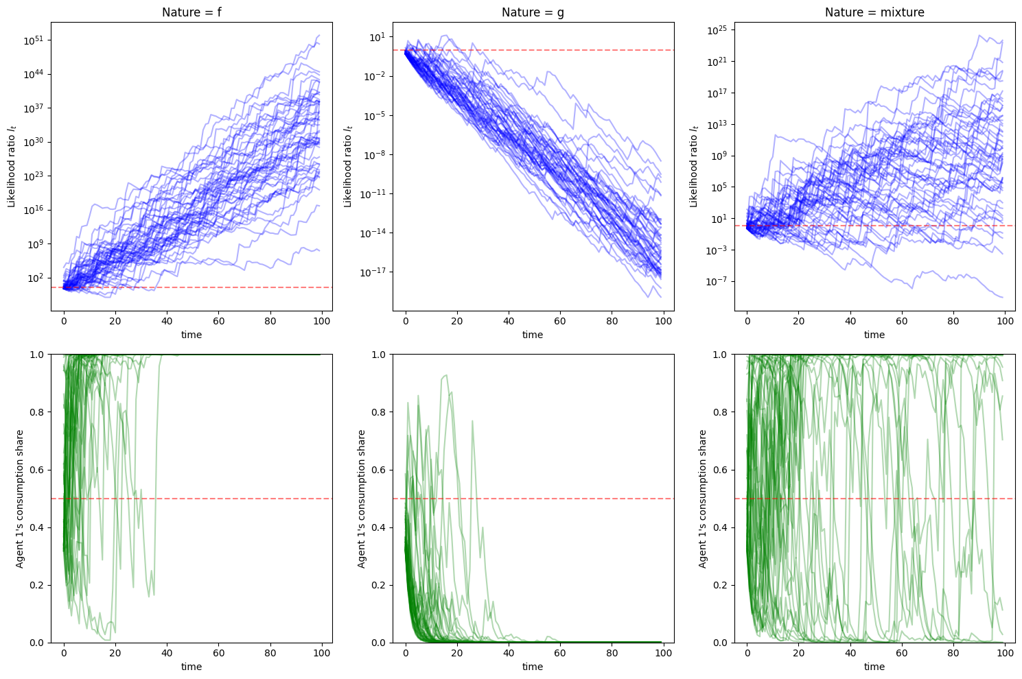
In the left panel, nature chooses $f$. Agent 1’s consumption reaches $1$ very quickly.

In the middle panel, nature chooses $g$. Agent 1’s consumption ratio tends to move towards $0$ but not as fast as in the first case.

In the right panel, nature flips coins each period. We see a very similar pattern to the processes in the left panel.

The figures in the top panel remind us of the discussion in this section.

We invite readers to revisit that section and try to infer the relationships among $D_{KL}(f\Vert g)$, $D_{KL}(g\Vert f)$, $D_{KL}(h\Vert f)$, and $D_{KL}(h\Vert g)$.

Let’s compute values of KL divergence

shares = [np.mean(c1_f[:, -1]), np.mean(c1_g[:, -1]), np.mean(c1_h[:, -1])]
Kf_g, Kg_f = compute_KL(f, g), compute_KL(g, f)
Kf_h, Kg_h = compute_KL_h(h, f, g)

print(f"Final shares: f={shares[0]:.3f}, g={shares[1]:.3f}, mix={shares[2]:.3f}")
print(f"KL divergences: \nKL(f,g)={Kf_g:.3f}, KL(g,f)={Kg_f:.3f}")
print(f"KL(h,f)={Kf_h:.3f}, KL(h,g)={Kg_h:.3f}")

Final shares: f=1.000, g=0.000, mix=0.928
KL divergences: 
KL(f,g)=0.759, KL(g,f)=0.344
KL(h,f)=0.073, KL(h,g)=0.281

We find that $KL(f,g)>KL(g,f)$ and $KL(h,g)>KL(h,f)$.

The first inequality tells us that the average “surprise” from having belief $g$ when nature chooses $f$ is greater than the “surprise” from having belief $f$ when nature chooses $g$.

This explains the difference between the first two panels we noted above.

The second inequality tells us that agent 1’s belief distribution $f$ is closer to nature’s pick than agent 2’s belief $g$.

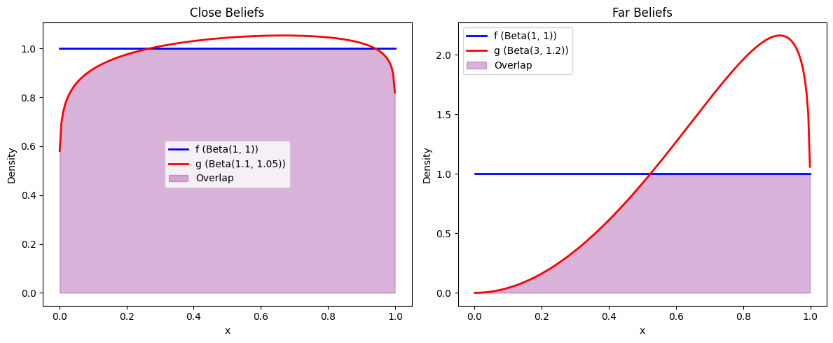
To make this idea more concrete, let’s compare two cases:

• agent 1’s belief distribution $f$ is close to agent 2’s belief distribution $g$;

• agent 1’s belief distribution $f$ is far from agent 2’s belief distribution $g$.

We use the two distributions visualized below

def plot_distribution_overlap(ax, x_range, f_vals, g_vals, 
                            f_label='f', g_label='g', 
                            f_color='blue', g_color='red'):
    """Plot two distributions with their overlap region."""
    ax.plot(x_range, f_vals, color=f_color, linewidth=2, label=f_label)
    ax.plot(x_range, g_vals, color=g_color, linewidth=2, label=g_label)
    
    overlap = np.minimum(f_vals, g_vals)
    ax.fill_between(x_range, 0, overlap, alpha=0.3, color='purple', label='Overlap')
    ax.set_xlabel('x')
    ax.set_ylabel('Density')
    ax.legend()
    
# Define close and far belief distributions
f_close = jit(lambda x: p(x, 1, 1))
g_close = jit(lambda x: p(x, 1.1, 1.05))

f_far = jit(lambda x: p(x, 1, 1))
g_far = jit(lambda x: p(x, 3, 1.2))

# Visualize the belief distributions
fig, (ax1, ax2) = plt.subplots(1, 2, figsize=(12, 5))

x_range = np.linspace(0.001, 0.999, 200)

# Close beliefs
f_close_vals = [f_close(x) for x in x_range]
g_close_vals = [g_close(x) for x in x_range]
plot_distribution_overlap(ax1, x_range, f_close_vals, g_close_vals,
                         f_label='f (Beta(1, 1))', g_label='g (Beta(1.1, 1.05))')
ax1.set_title(f'Close Beliefs')

# Far beliefs
f_far_vals = [f_far(x) for x in x_range]
g_far_vals = [g_far(x) for x in x_range]
plot_distribution_overlap(ax2, x_range, f_far_vals, g_far_vals,
                         f_label='f (Beta(1, 1))', g_label='g (Beta(3, 1.2))')
ax2.set_title(f'Far Beliefs')

plt.tight_layout()
plt.show()

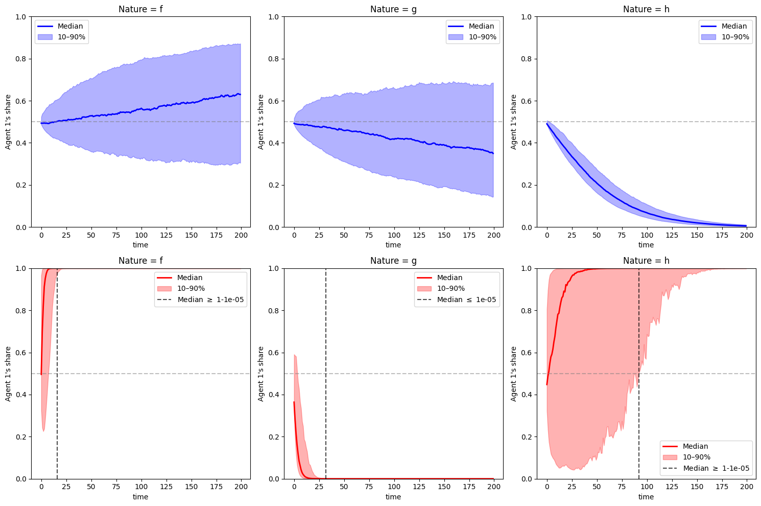
Let’s draw the same consumption ratio plots as above for agent 1.

We replace the simulation paths with median and percentiles to make the figure cleaner.

Staring at the figure below, can we infer the relation between $KL(f,g)$ and $KL(g,f)$?

From the right panel, can we infer the relation between $KL(h,g)$ and $KL(h,f)$?

fig, axes = plt.subplots(2, 3, figsize=(15, 10))
nature_params = {'close': [(1, 1), (1.1, 1.05), (2, 1.5)],
                 'far':   [(1, 1), (3, 1.2),   (2, 1.5)]}
nature_labels = ["Nature = f", "Nature = g", "Nature = h"]
colors = {'close': 'blue', 'far': 'red'}

threshold = 1e-5  # "close to zero" cutoff

for row, (f_belief, g_belief, label) in enumerate([
                        (f_close, g_close, 'close'),
                        (f_far, g_far, 'far')]):
    
    for col, nature_label in enumerate(nature_labels):
        params = nature_params[label][col]
        s_seq = np.random.beta(params[0], params[1], (1000, 200))
        _, c1 = simulate_blume_easley(s_seq, f_belief, g_belief, λ)
        
        median_c1 = np.median(c1, axis=0)
        p10, p90 = np.percentile(c1, [10, 90], axis=0)
        
        ax = axes[row, col]
        color = colors[label]
        ax.plot(median_c1, color=color, linewidth=2, label='Median')
        ax.fill_between(range(len(median_c1)), p10, p90, alpha=0.3, color=color, label='10–90%')
        ax.set_xlabel('time')
        ax.set_ylabel("Agent 1's share")
        ax.set_ylim([0, 1])
        ax.set_title(nature_label)
        ax.axhline(y=λ, color='gray', linestyle='--', alpha=0.5)
        below = np.where(median_c1 < threshold)[0]
        above = np.where(median_c1 > 1-threshold)[0]
        if below.size > 0: first_zero = (below[0], True)
        elif above.size > 0: first_zero = (above[0], False)
        else: first_zero = None
        if first_zero is not None:
            ax.axvline(x=first_zero[0], color='black', linestyle='--',
                       alpha=0.7, 
                       label=fr'Median $\leq$ {threshold}' if first_zero[1]
                       else fr'Median $\geq$ 1-{threshold}')
        ax.legend()

plt.tight_layout()
plt.show()

Holding to our guesses, let’s calculate the four values

# Close case
Kf_g, Kg_f = compute_KL(f_close, g_close), compute_KL(g_close, f_close)
Kf_h, Kg_h = compute_KL_h(h, f_close, g_close)

print(f"KL divergences (close): \nKL(f,g)={Kf_g:.3f}, KL(g,f)={Kg_f:.3f}")
print(f"KL(h,f)={Kf_h:.3f}, KL(h,g)={Kg_h:.3f}")

# Far case
Kf_g, Kg_f = compute_KL(f_far, g_far), compute_KL(g_far, f_far)
Kf_h, Kg_h = compute_KL_h(h, f_far, g_far)

print(f"KL divergences (far): \nKL(f,g)={Kf_g:.3f}, KL(g,f)={Kg_f:.3f}")
print(f"KL(h,f)={Kf_h:.3f}, KL(h,g)={Kg_h:.3f}")

KL divergences (close): 
KL(f,g)=0.003, KL(g,f)=0.003
KL(h,f)=0.073, KL(h,g)=0.061
KL divergences (far): 
KL(f,g)=0.759, KL(g,f)=0.344
KL(h,f)=0.073, KL(h,g)=0.281

We find that in the first case, $KL(f,g)\approx KL(g,f)$ and both are relatively small, so although either agent 1 or agent 2 will eventually consume everything, convergence displayed in the first two panels on the top is pretty slow.

In the first two panels at the bottom, we see convergence occurring faster (as indicated by the black dashed line) because the divergence gaps $KL(f,g)$ and $KL(g,f)$ are larger.

Since $KL(f,g)>KL(g,f)$, we see faster convergence in the first panel at the bottom when nature chooses $f$ than in the second panel where nature chooses $g$.

This ties in nicely with (22.1).

23.10. Related Lectures#

Likelihood processes play an important role in Bayesian learning, as described in Likelihood Ratio Processes and Bayesian Learning and as applied in Job Search VII: Search with Learning.

Likelihood ratio processes appear again in Additive and Multiplicative Functionals.

23.11. Exercise#